December 4, 2023
The A/B Testing Playbook For Mobile Games, Part 2: Statistical Significance Testing

In the first article in this series: The A/B Testing Playbook for Mobile Games, Part 1: Structuring the Experiment, we discussed the different types of A/B testing (also known as “split-testing”), how to properly structure experiments, and the most common mistakes my team has seen in our work with 90+ mobile game studios.
In this article, we’ll dig into the mechanics of the one statistical tool that we use most frequently in split-test analysis.

⚠️ Caution: Statistical significance testing can be very dangerous when used without an adequate understanding of why and how it works. As a product manager (not a statistician) by trade with over 750 split-tests under my belt, I have intimate experience with being on the wrong side of these mistakes 🤦♂️. So, in this article I’ll attempt to provide the necessary background on the statistics while keeping things as simple as possible for the non-statisticians out there (including yours truly).
Statistical Significance, Made Simple(ish)
When split-testing changes to our game, what we really want to know is:

Unfortunately, predicting the future is a messy business.
The best we can do is use the behavior of a small player sample, paired with statistical analysis, to place bets about the potential behavior of the broader population (i.e. all current and future players) once exposed to our change. This helps us make product choices with a higher rate of success than if we operated on intuition alone.
To gain valuable insights from split-testing, we need to set up experiments correctly, and then analyze them correctly (a nontrivial task!):
Step 1: Execute a split-test. Expose different player samples to different treatments of your game, let them play for a predefined period of time, then measure differences in average KPI (or lever metric) between player samples.
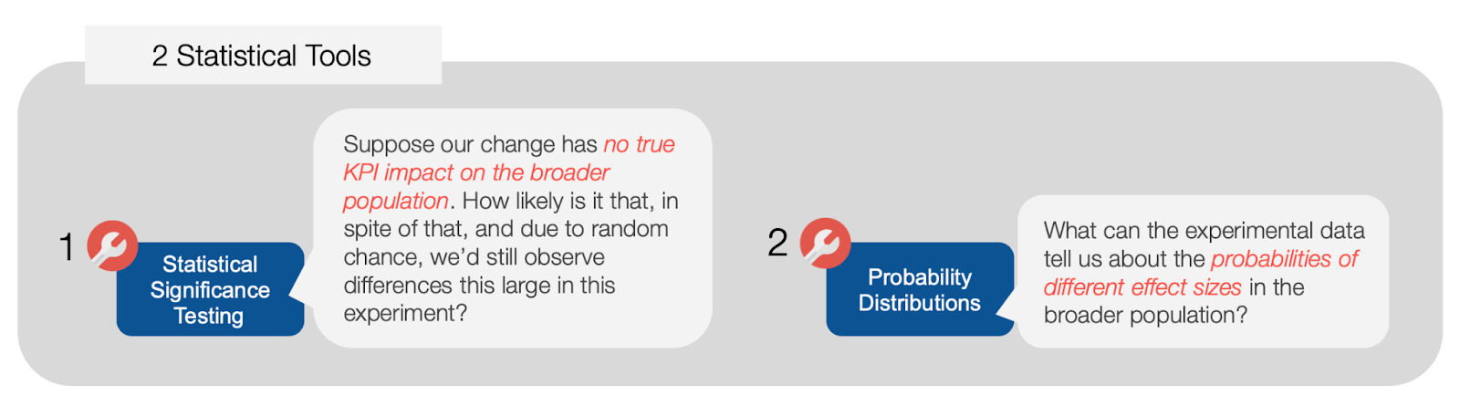
Step 2: IF we observe meaningful KPI differences between our player samples, we can use two statistical tools to predict the true KPI change for the broader population in response to our game changes:
- Statistical Significance Testing, and
- Probability Distributions
Key Terms to Know
- Player sample: A relatively small, randomly selected group of players whose behavior we will analyze directly, typically to make predictions about the behavior of the broader population.
- Broader population: An unmeasurable group that includes ALL current and future players. In inferential statistics, we analyze a small sample of players in order to make inferences or predictions about the behavior of the broader population.
- Treatments: Often called “variants.” The different variations of your game that you wish to split-test. Typically you will have a control group, and one or more alternate treatments.
- Control group: The set of players who experience no game changes (in other words, they experience the “normal” version of the game), and whose KPI we analyze against those of the player sample in order to detect a change.
- KPI: (Key Performance Indicator) A small group of summary metrics that serve as final aggregates (typically averages) for diverse types of behavior. The canonical examples are ARPU (average revenue per user) and dX Retention (day 1, 7, 30 retention).
Know Thy Enemy: Sampling Error

Within any randomly chosen player sample, and behind any KPI expressed as an average (as most are), lurks a LOT of internal variation in player behavior.
Most confounding is the case of IAP spend in F2P games, where it is typical for a random sample of 1,000 players to contain 950 players with $0 spend, such that ARPU is shaped by a mere handful of minnows, dolphins and whales. For example:
| Players in Sample | D365 Gross ARPU |
| 950 | $0 |
| 45 | $20 |
| 3 | $100 |
| 1 | $500 |
| 1 | $2,000 |
| Average | $3.70 |
Presented as an average, this entire sample’s ARPU (average revenue per user) is $3.70. However, this is a tremendous and uncomfortable amount of variation to bury in an average. Because two individual users’ behavior can be so wildly different ($0 vs. $2,000), the random selection of players, for our small sample, has a dramatic impact on the sample average.
If a second whale (say a $1,000 player) was randomly included in our 1000-player sample, sample ARPU would increase by a whopping 54% to $5.70, not because of any game change we made, but merely due to random sampling error.
Sampling error, for our purposes, can be defined as the difference between the KPI (e.g. ARPU) observed in a small player sample, and the true KPI for the broader population the sample is meant to represent.
Sampling error, results from the fact that, and to the extent that, a small sample of players overweights or underweights certain behaviors depending on who is or isn’t randomly included in the sample. If the broader population has 1% whales, and your sample randomly happens to contain 2%, you are likely to experience significant sampling error due to the overrepresentation of whales and their spend in the sample. This is also why increasing your sample sizes reduces the impact of sampling error. If we have a 10,000-player sample with 10 whales, then including one additional whale in the random sample is less distorting than was the case in our 1,000-player sample.
So, if we run an experiment, hoping to lift ARPU, what might give us confidence that an ARPU lift observed in the experimental treatment (relative to the control treatment) was real, and not the result of sampling error?
To confidently say that our product changes caused the observed ARPU increase, we’d want to observe a positive ARPU change much larger, and/or more broadly distributed across players in the sample, than could reasonably be expected from sampling error.
Another way of framing this: we’re looking for a signal that so greatly exceeds the level of likely noise that it convinces us that the KPI change we observed is almost certainly the direct result of our game changes.
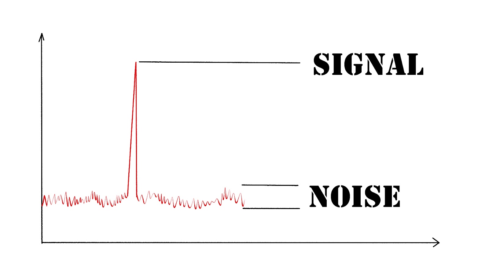
To compare signal to noise, we’ll need to use a statistical significance test.
Welch’s T-Test 🍇
If you research statistical significance testing, you’ll find an intimidating number of specialized methods and techniques.
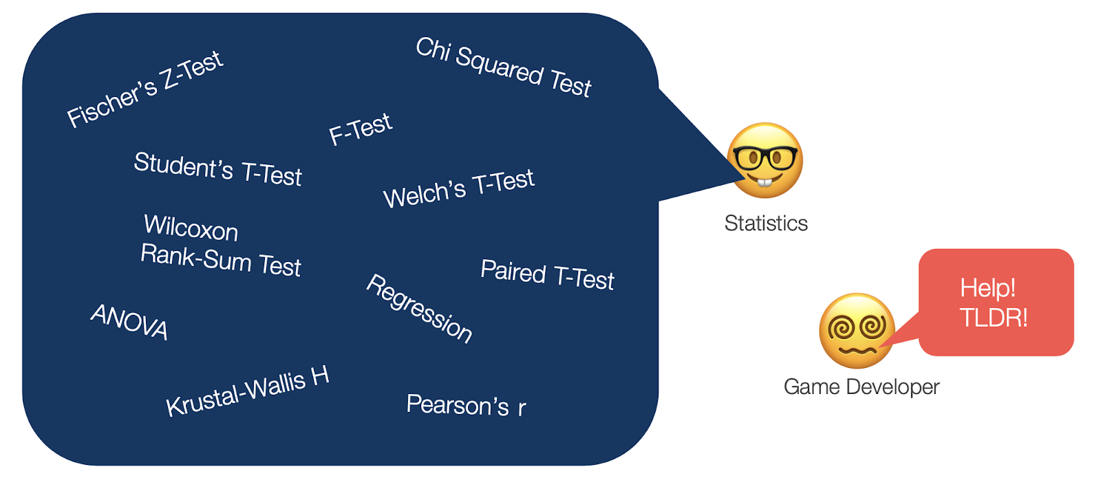
Luckily, for mobile game split-testing, we can nearly always rely on Welch’s T-Test, aka the “unequal variances t-test.”
Why? This test is appropriate for any split-test where all the following are true:
- we randomly assign users to independent groups,
- we’re comparing KPI, expressed as averages, between samples, and
- we’re not certain that all samples have identical size and variance (defined below)
The Welch’s (unequal variances) t-test can be easily performed in Excel or Google Sheets, but let’s stay focused on comprehension for now.
“t”, the Test Statistic
Welch’s T-Test compares two data samples and generates a “t” value, often called a “test statistic”.
The “test statistic” is an abstract concept (bordering on pedantic to non-statisticians), but I find it useful to think of t as a simple ratio comparing statistical signal to noise.
For example:
- Signal: difference in D30 ARPU between two player samples
- Noise: “variance”: the random variation in spend values amongst the players in both samples.
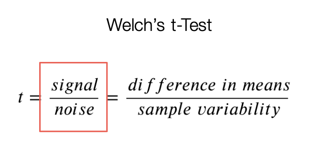
t is “strength of the difference observed, net noise”.
Let’s use another example to make this more concrete.
Analysis Example with Dummy Test Data
As a hypothetical exercise, let’s use Welch’s T-Test to evaluate an ARPU data set from a hypothetical experiment.
This data reflects a typical, painfully skewy F2P ARPU distribution where only 3% of players spend, and ARPU is heavily influenced by a small number of whales.
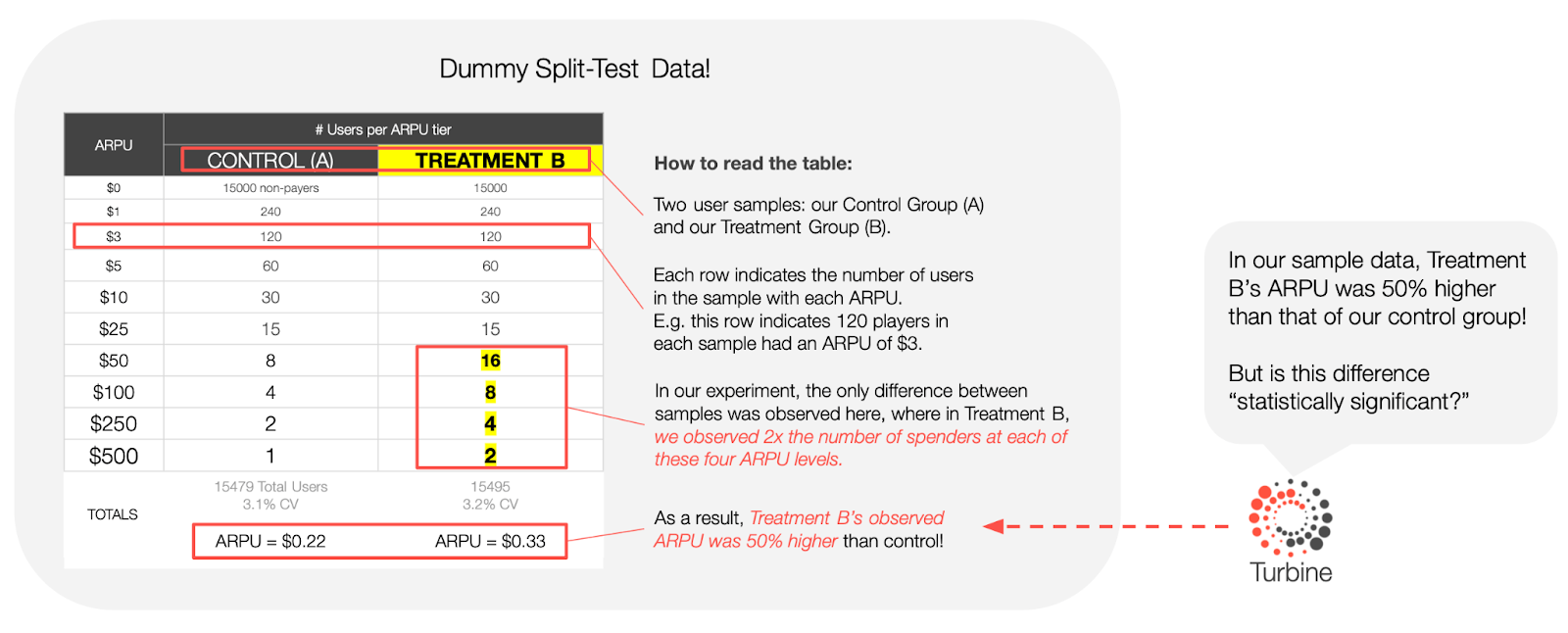
In our example experiment data above, Treatment B had 50% higher ARPU than the control group. Let’s use Welch’s t-test to compare that positive signal to the level of noise in the data so that we can determine how excited we should be about the observed results.
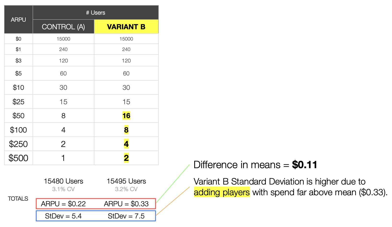
First we will calculate the difference in means between the samples for the KPI we are measuring (ARPU). Then, to fill in the denominator in the equation (“noise”), we will calculate the standard error using the standard deviations from our two samples.
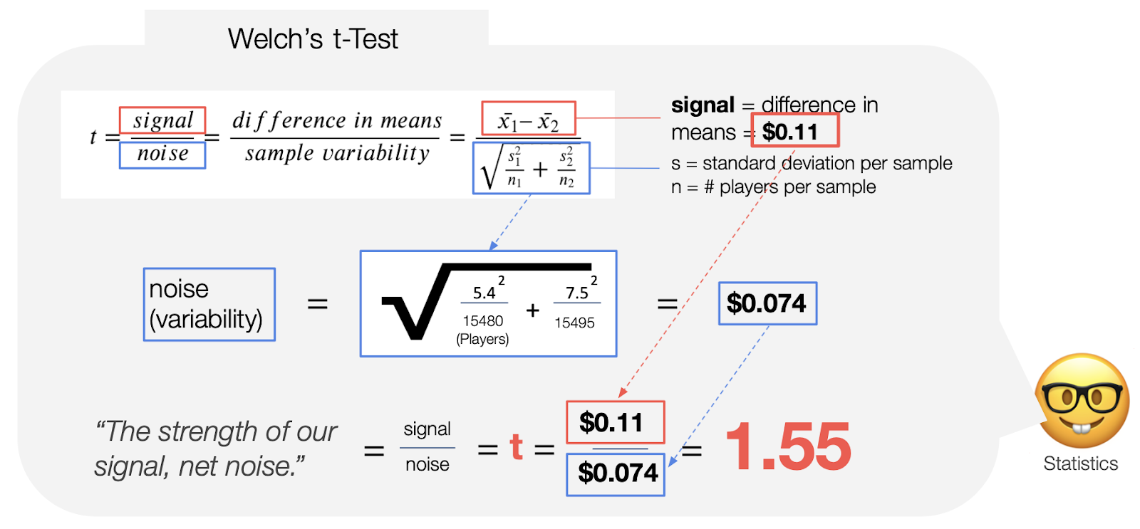
As we can see above, Welch’s 🍇 t-test yielded a t-value of 1.55 for our experiment.
What the Heck is a t-Value?

The t statistic has one job: to measure strength of evidence against the null hypothesis.
The null hypothesis is the possibility that, in the broader population, the true ARPU lift is zero.
In other words, the null hypothesis states that there’s “nothing to see here” because, after considering the level of ARPU variance within our samples, the observed ARPU difference between the control and variant treatments can easily be explained by sampling error.
So if the null hypothesis is true, we should not expect the 50% ARPU lift to be “reproducible”
(to produce similarly exciting results) in either a repeat experiment, OR in a full rollout to the broader population.
So, how do we use the t statistic to measure the strength of our evidence against the null hypothesis?
The T-Distribution
To use the t statistic to evaluate the null hypothesis, we unfortunately must contend with yet another abstraction: a probability curve called a t distribution.

A t-distribution is a probability distribution that helps us find the probability of getting a t value (i.e signal to noise ratio) this extreme, under the null hypothesis.
Where does this curve come from? Well, actually, from a Head Brewer at Guiness who was just trying to make a better beer, but that’s a story for another day. For our purposes, just understand that, the t curve is always the same for any given sample size (e.g. 1,000 users), such that the t-distribution curve essentially functions as a lookup table for P, given t.
Nerd bonus: 🤓 The t-distribution curve is always the same shape, except that it grows narrower and taller as sample size increases. With sample sizes in the thousands of users though, the change in shape is hardly detectable.
But I digress… what’s important is that we use our t-value (1.55 in our example), and the t probability distribution curve, to look up the value of P for our experiment.
P is the probability that, under the null hypothesis, sampling error could still cause us to get a t-value this high (or higher).

Wait, What the Heck is a P-Value? 😭
Right, let’s try again… P is the probability of observing a KPI change as large and as distributed (across players, instead of just concentrated on 1-2 whales), as the one we observed, entirely due to sampling error.
If our observed KPI change were due to sampling error, this would be bad for us, since it would suggest that our experimental change would fail to actually lift ARPU when rolled out to the broader population.
This probability P is also called the “P value.” In our case, the t-distribution for our sample size, with a t-value of 1.55, yields a P-value of 0.12 or 12%.
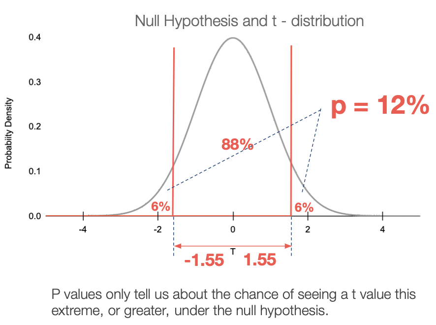
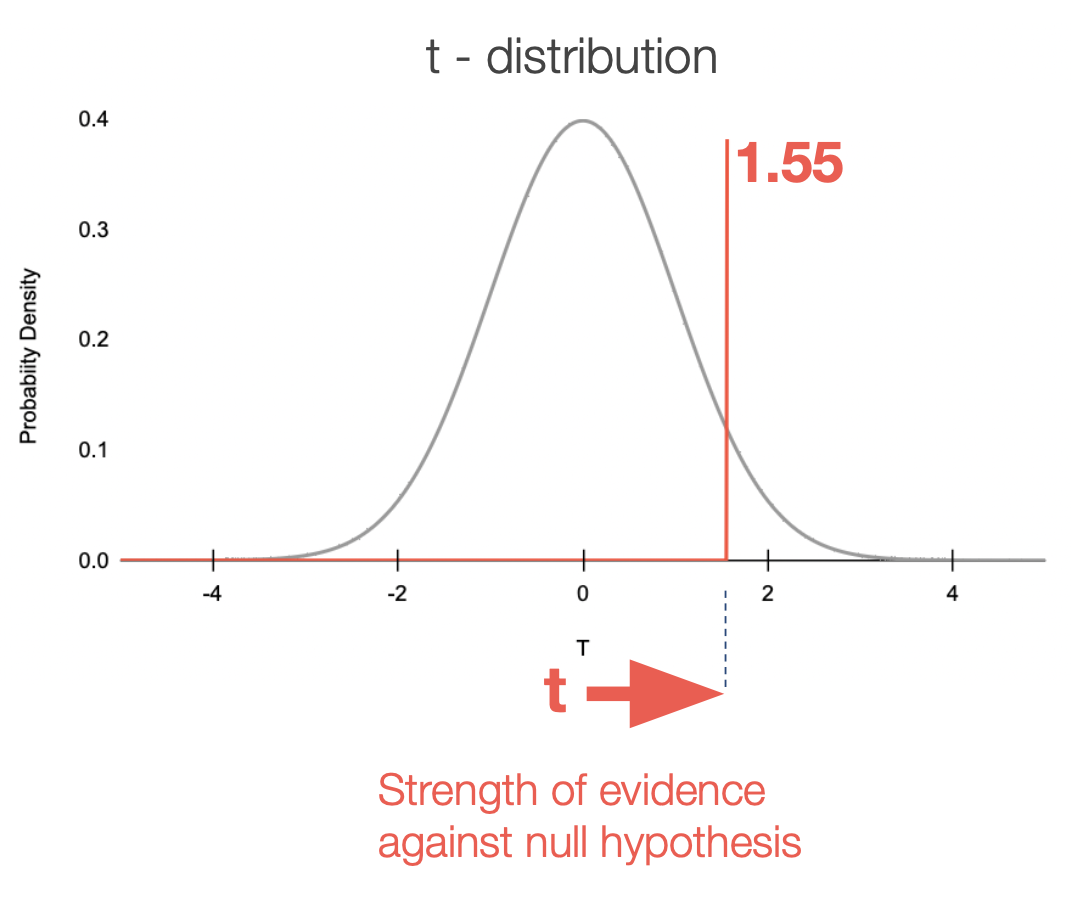
Nerd bonus: 🤓 The t probability distribution curve above illustrates the probabilities of getting different t values under the null hypothesis. The x-axis is t. The y-axis is the probability at each point on the curve. The total area under the curve represents 100% of possible outcomes. As you can see, higher t values are less and less probable (lower y-axis values). The area under the curve in both directions, beyond our t values of t = 1.55 or t = -1.55 is the P value for our experiment = 12%.
Mega-nerd bonus: 🤓 Curious why we must evaluate t = -1.55 when our t-value was positive 1.55? That’s a particularly tortuous question, but the short answer is that we’re treating this as a “two-sided” analysis, and looking for values “as extreme” as 1.55, which implies distance from 0 in both positive and negative directions.
So, What can we conclude from P = 12%?
So, what p = 12% explicitly tells us is: if our product changes have no true KPI impact, we’d still have a ~12% chance of observing an ARPU lift this extreme due to sampling error alone.
And, at the risk of beating a dead horse, this would suggest a 12% chance that the cause of our ARPU bump was (perhaps) catching an extra whale or two in our random sample of 1,000 players.
More explicitly, p = 12% projects a 12% chance of getting a t-value of 1.55 or higher due to sampling error. So if we ran this experiment 100 times (with player samples of similar size and variance) but we changed the experiment so that the variant and control groups had identical game treatments (i.e. no game changes), we should still expect to get a t value >= 1.55 in 12 out of those 100 experiments just by dumb luck.
Scientific convention is to look for p values of 5% or lower to declare an experimental outcome to be statistically significant. So, our 12% wouldn’t strictly qualify, and it follows that the 50% ARPU lift we observed can’t be considered statistically significant in the formal sense.
BUT, a p-value of 12% does imply that the variant is significantly more likely than not to have the higher “true” ARPU, and therefore I would caution against automatically rejecting the variant.
To make a sensible decision, we’ll want to weigh other considerations alongside the p-value to make a comprehensive decision. This is where experience both running experiments and understanding your users can be invaluable.
To thoughtfully conclude this experiment, I might consider the following:
- P-value: P = 12% implies it’s more likely than not that the variant has higher true ARPU, BUT…
- Technical risk: How risky is it that we screw something up (e.g. introduce bugs) when rolling this out?
- Player sentiment risk: Does this change run the risk of upsetting players?
- New vs. existing users: How might this change impact newer vs. elder players differently? Do we need to test both?
- Probability distribution of effect size: How much lift should we expect, and does it justify the risks? (see next article!)
- Assessing known priors:
- Have we tested similar changes in the past? How were the results?
- Have our competitors made this change? How confident are we that they tested it and proved it successful, and how similar are our players?
- Level of trust in experiment: How confident are we in the reliability of how we structured the experiment, and collected data?
This is where making a decision about whether and how to roll out a tested change is as much art as science. The p-value is a valuable (and essential) input to this decision, but by no means should it be the only consideration. Trust me on this one, as I’ve learned this the hard way through hundreds of split-tests on live games.
What P doesn’t tell us: How large is our effect?
One limitation of the P value is that it tells us very little about what magnitude of effect sizes we can expect in the broader population.
This is limiting, because, as game developers, what we really want to know is:
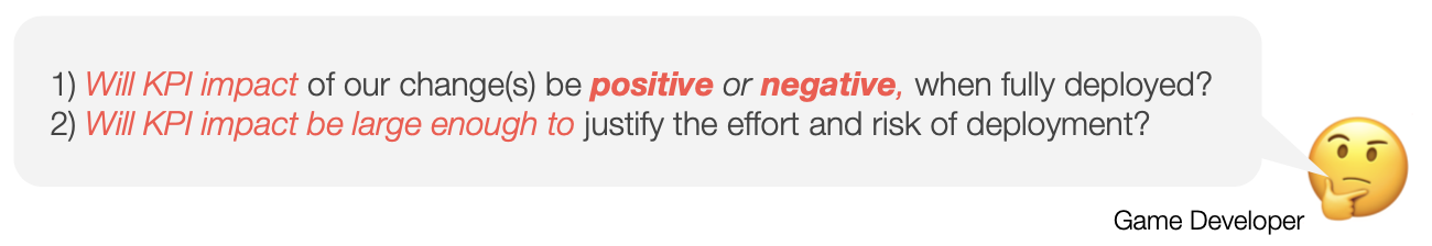
Suppose that in a split-test we observe an ARPU lift of 33%, and a p-value of 5%, suggesting that this is a “statistically significant impact.”
A p-value of 5% does not suggest that we should expect a 33% ARPU lift when rolling out this treatment.
Instead, by producing a p-value of 5%, the (large) observed 33% ARPU lift helped convince us that the treatment is very likely to produce a higher ARPU in the broader population.
But how much higher? Suppose we wanted an ARPU lift of at least 10% to justify the risk of proceeding with the variant. How might we find the probability of a >= 10% true lift?
This brings us to a discussion of our second statistical tool, which we’ll discuss in the next article: effect sizes!
In the next article in this series, The A/B Testing Playbook for Mobile Games, Part 3: Probability Distribution of Effect Size, we’ll go deep on our second statistical tool for analyzing split-test results.
As always, if you have questions, comments, or critiques, I want to hear them! And if you’re interested in deploying rapid and reliable split-testing for your game, I would love to help: matt@turbine.games.
If you enjoyed this article, you might also like my series on F2P IAP Merchandising best practices:
- The IAP Merchandising Playbook, Part 1: Special Offers That Sizzle
- The IAP Merchandising Playbook, Part 2: Visual Hierarchy
- The IAP Merchandising Playbook, Part 3: MVP Store Design
Need help with your game? Email me at matt@turbine.games, or book a time on my calendar.
Turbine helps mobile game & app publishers drive UA and product KPIs.
Book Intro Call